From marginal effects to meaningful moderator interpretation
Disclaimer: All data used in this chapter is simulated and does not reflect real-world data. The purpose of this chapter is to illustrate the concept of interaction terms in linear regression models, not to make any claims about the relationship between age, income, and ideological placement.
4.1 Interaction Terms as Context
“If You Are Not a Liberal at 25, You Have No Heart. If You Are Not a Conservative at 35 You Have No Brain”
Researchers often want to know whether relationships differ across contexts. I use ideological self-placement as the running example. More specifically, I want to know whether age affects left-right self-placement. In addition, I assume that income affects ideological leanings as well, meaning that voters at the lower end of the income distribution are typically more left than voters on the higher end of the income distribution. So, how can interaction terms help us understand the relationship between age, income and ideological placement? Does the relationship between age and ideological placement differ across income levels? If so, how can I model this relationship?
4.2 What is an Interaction Term?
In this example, income is measured in tens of thousands, and leftRight is a 0-10 self-placement scale where higher values indicate more right-leaning views. The simulated data are generated with the following true parameters: the baseline effect of age on ideology is \(\beta_1 = 0.02\), the main effect of income is \(\beta_2 = 0.15\), and the interaction is \(\beta_3 = 0.004\). This means the true marginal effect of age on left-right placement is \(0.02 + 0.004 \times income\), so the age effect increases by 0.004 for each additional unit of income.
I established in the previous chapter that a coefficient in a regression model represents the average effect of a predictor variable on the response variable, holding all other variables constant. However, this assumes that the effect of the predictor is the same across all contexts. Using a linear regression model with a continuous response variable leftRight and a predictor variable age, I can illustrate this point. Mathematically, our model without an interaction term looks as follows:
Equation 4.1 shows that the marginal effect of a predictor variable in a linear regression model is represented by the coefficient \(\beta_1\). To understand interactions, it is helpful to know that the marginal effect of a predictor can be read directly from the equation because it is the partial derivative of the response variable with respect to the predictor variable. In our simple regression model, the marginal effect of age is \(\beta_1\), which means that for every one-unit increase in age, the expected change in leftRight is \(\beta_1\) units. Mathematically, the partial derivative of Equation 4.1 can be expressed as: \[
\frac{\partial leftRight_i}{\partial age_i} = \beta_1
\tag{4.2}\]
In R, this model can be estimated using the lm() function as follows:
summary(lm(leftRight ~ age, data = data))
Call:
lm(formula = leftRight ~ age, data = data)

Residuals:
    Min      1Q  Median      3Q     Max
-3.5059 -0.8757 -0.0084  0.9727  3.0922

Coefficients:
            Estimate Std. Error t value Pr(>|t|)
(Intercept) 3.697214   0.118956   31.08   <2e-16 ***
age         0.045269   0.002289   19.78   <2e-16 ***
---
Signif. codes:  0 '***' 0.001 '**' 0.01 '*' 0.05 '.' 0.1 ' ' 1

Residual standard error: 1.289 on 998 degrees of freedom
Multiple R-squared:  0.2816,    Adjusted R-squared:  0.2809
F-statistic: 391.3 on 1 and 998 DF,  p-value: < 2.2e-16
So, why is this important to understand interaction terms? An interaction term is essentially a multiplicative combination of two predictor variables. When I include an interaction term in the regression model, I simply add two predictors and their product to the equation. Let’s assume that I want to know whether the effect of age on leftRight depends on the income of a respondent. Our regression model with the interaction term would look like this: \[
leftRight_i = \alpha + \beta_1 age_i + \beta_2 income_i + \beta_3 (age_i \times income_i) + \epsilon_i
\tag{4.3}\]
If I take the partial derivative of Equation 4.3 with respect to age, I get: \[
\frac{\partial leftRight_i}{\partial age_i} = \beta_1 + \beta_3 income_i
\tag{4.4}\]
As Equation 4.4 shows, the effect of age on leftRight is no longer constant but depends on the value of income. The coefficient \(\beta_3\) represents the change in the effect of age for each one-unit increase in income. If \(\beta_3\) is positive, it means that the effect of age on leftRight increases as income increases. Conversely, if \(\beta_3\) is negative, it means that the effect of age on leftRight decreases as income increases.
In R, this would look like this:
summary(lm(leftRight ~ age * income, data = data))
Call:
lm(formula = leftRight ~ age * income, data = data)

Residuals:
     Min       1Q   Median       3Q      Max
-2.45589 -0.55774  0.02019  0.56182  2.66821

Coefficients:
             Estimate Std. Error t value Pr(>|t|)
(Intercept) 2.4255133  0.2030559  11.945  < 2e-16 ***
age         0.0224525  0.0038078   5.896 5.08e-09 ***
income      0.1625065  0.0264208   6.151 1.12e-09 ***
age:income  0.0037022  0.0005002   7.401 2.86e-13 ***
---
Signif. codes:  0 '***' 0.001 '**' 0.01 '*' 0.05 '.' 0.1 ' ' 1

Residual standard error: 0.8063 on 996 degrees of freedom
Multiple R-squared:  0.7196,    Adjusted R-squared:  0.7187
F-statistic: 851.9 on 3 and 996 DF,  p-value: < 2.2e-16
(R adds the constitutive terms automatically when you use the * operator between two variables in the formula.)
The Interaction Coefficient Is Not the Full Story
The coefficient on the interaction term (\(\hat\beta_3\)) tells you the rate of change of the marginal effect, not the marginal effect itself. The marginal effect of age at any given income level is \(\hat\beta_1 + \hat\beta_3 \times income\). Always compute and visualize the full marginal effect across the moderator’s range rather than interpreting \(\hat\beta_3\) in isolation.
Even though it is more informative to plot the interaction to understand how the effect of age changes across different income levels, I can also look at the coefficients to get a sense of the interaction. First, I can see that the coefficient for age is positive. However, the coefficient for age gives us only the effect of age when income is zero, which is not a meaningful value in this context. A solution here would be to center the income variable around its mean before including it in the regression model. This way, the coefficient for age would represent the effect of age at the average income level.
On Centering Predictors
Centering continuous predictors before including them in interaction models serves two purposes: (1) it makes the constitutive terms (\(\hat\beta_1\), \(\hat\beta_2\)) directly interpretable at the mean of the other variable rather than at zero, and (2) it can reduce multicollinearity between the interaction term and its constitutive terms, improving numerical stability. Centering does not change the interaction coefficient, the marginal effects, or the model fit but only the interpretation of the lower-order coefficients.
Second, the coefficient for the interaction term age:income is positive, which indicates that the effect of age on leftRight increases as income increases. This means that age is more strongly associated with rightward placement among higher-income respondents than among lower-income respondents. Therefore, the table alone already gives us a pretty good idea of the interaction, but it is often more intuitive to visualize it:
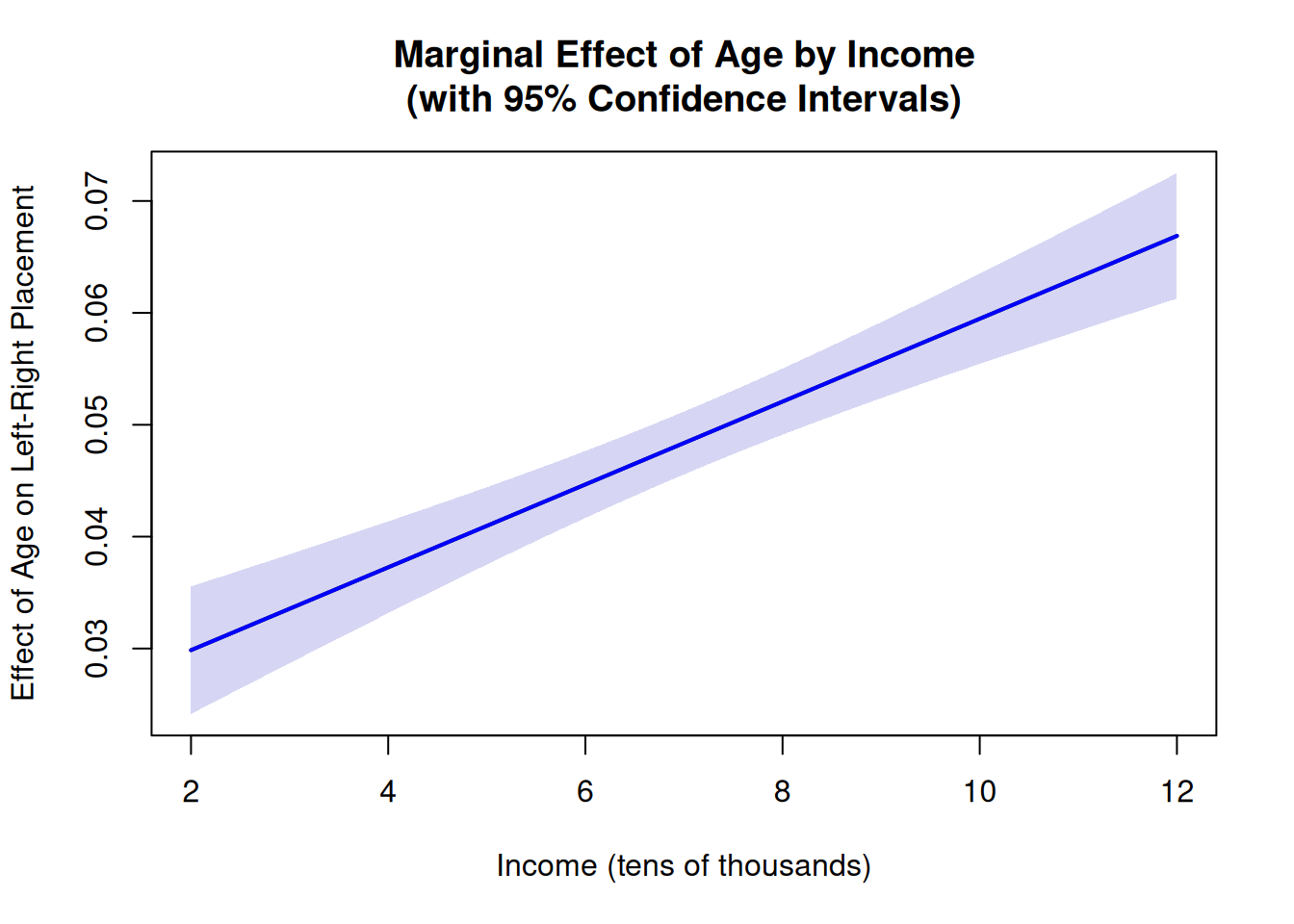
# Fit the model with interactionmodel <-lm(leftRight ~ age * income, data = data)# Extract coefficients and variance-covariance matrixcoefs <-coef(model)vcov_matrix <-vcov(model)income_seq <-seq(2, 12, length.out =100)effect <- coefs[2] + coefs[4] * income_seqse <-sqrt(vcov_matrix[2, 2] + income_seq^2* vcov_matrix[4, 4] +2* income_seq * vcov_matrix[2, 4])ci_lower <- effect -1.96* seci_upper <- effect +1.96* se# Create plotplot(income_seq, effect, type ="l", lwd =2,ylim =c(min(ci_lower), max(ci_upper)),xlab ="Income (tens of thousands)",ylab ="Effect of Age on Left-Right Placement",main ="Marginal Effect of Age by Income\n(with 95% Confidence Intervals)")# Add confidence interval as shaded regionpolygon(c(income_seq, rev(income_seq)), c(ci_upper, rev(ci_lower)),col =rgb(0.2, 0.2, 0.8, 0.2),border =NA)# Add reference line at y=0abline(h =0, lty =2, col ="gray", lwd =1)# Re-plot the line on toplines(income_seq, effect, lwd =2, col ="blue")
Figure 4.1: Marginal effect of age on left-right placement across income levels. The effect is positive throughout the observed income range but increases with income.
To plot the marginal effect of age on leftRight across different income levels, along with 95% confidence intervals, I use the coefficients and variance-covariance matrix from the fitted model. To compute variance for the confidence intervals, I apply the delta method:
The plot shows that the estimated effect of age is positive across the observed income range. This visualization gives us a much clearer picture of how the effect of age changes across income levels compared to a regression table. While age increases rightward placement for all income levels, the effect is much stronger for higher-income respondents than for lower-income respondents.
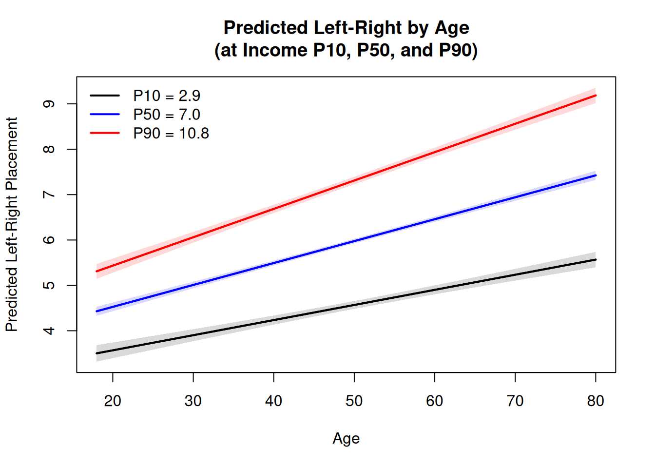
An alternative way to visualize the interaction is to plot predicted values of leftRight across age for different income levels. To do so, I use the 10%, 50%, and 90% quantiles of the income variable to represent low, medium, and high income levels, respectively. I then plot the predicted leftRight values across age for these three income levels, along with confidence intervals.
Figure 4.2: Predicted left-right placement by age at the 10th, 50th, and 90th percentiles of income. The steeper slope for higher income illustrates the positive interaction.
The plot shows that the predicted leftRight values increase with age for all three income levels, but the slope is steeper for higher-income respondents. This visualization provides an alternative way to understand how the relationship between age and leftRight changes across different income levels, compared to the previous plot of marginal effects. Which visualization is more informative depends on the research question and the audience.
4.3 A Brief Digression: Polynomial Regression
I now extend the interaction idea to nonlinearity. In an interaction, the slope of one variable changes with another variable (x × z). With polynomial terms, the slope of a variable changes with its own level by including powers like x² and x³. Although both are multiplicative in form, polynomial terms are conventionally treated as predictor transformations (basis expansions), not as interaction terms. Using age as an example, our regression model with a cubic term would look like this: \[
leftRight_i = \alpha + \beta_1 age_i + \beta_2 age_i^2 + \beta_3 age_i^3 + \epsilon_i
\tag{4.5}\]
The partial derivative of Equation 4.5 with respect to age is: \[
\frac{\partial leftRight_i}{\partial age_i} = \beta_1 + 2 \beta_2 age_i + 3 \beta_3 age_i^2
\tag{4.6}\]
In R, a polynomial regression can be estimated by either using the poly() function (or including the polynomial terms manually) as follows:
summary(lm(leftRight ~poly(age, degree =3, raw =TRUE), data = data2))
Call:
lm(formula = leftRight ~ poly(age, degree = 3, raw = TRUE), data = data2)

Residuals:
     Min       1Q   Median       3Q      Max
-2.25298 -0.55461  0.01145  0.54104  2.61350

Coefficients:
                                     Estimate Std. Error t value Pr(>|t|)
(Intercept)                         3.510e+00  5.398e-01   6.502 1.25e-10 ***
poly(age, degree = 3, raw = TRUE)1  1.861e-01  3.825e-02   4.865 1.33e-06 ***
poly(age, degree = 3, raw = TRUE)2 -3.574e-03  8.315e-04  -4.298 1.89e-05 ***
poly(age, degree = 3, raw = TRUE)3  2.323e-05  5.631e-06   4.126 4.00e-05 ***
---
Signif. codes:  0 '***' 0.001 '**' 0.01 '*' 0.05 '.' 0.1 ' ' 1

Residual standard error: 0.8007 on 996 degrees of freedom
Multiple R-squared:  0.1354,    Adjusted R-squared:  0.1328
F-statistic:    52 on 3 and 996 DF,  p-value: < 2.2e-16
And the plot of the marginal effect of age on leftRight would look like this:
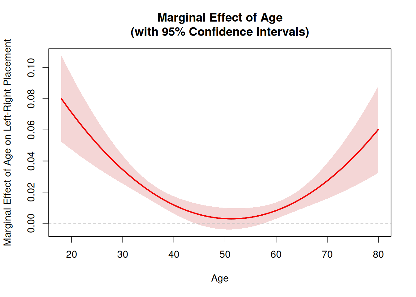
# Fit the polynomial regression model with raw polynomialsmodel_poly <-lm(leftRight ~ age +I(age^2) +I(age^3), data = data2) # Extract coefficients and variance-covariance matrixcoefs <-coef(model_poly)vcov_matrix <-vcov(model_poly)# Create age sequence for predictionage_seq <-seq(18, 80, length.out =100)# Calculate marginal effect: β₁ + 2*β₂*age + 3*β₃*age²effect <- coefs[2] +2* coefs[3] * age_seq +3* coefs[4] * age_seq^2# Delta method for standard error:# For f(β) = β₁ + 2*β₂*age + 3*β₃*age², gradient is [1, 2*age, 3*age²]# SE = sqrt(gradient' * Vcov * gradient)se <-sqrt(vcov_matrix[2, 2] +4* age_seq^2* vcov_matrix[3, 3] +9* age_seq^4* vcov_matrix[4, 4] +4* age_seq * vcov_matrix[2, 3] +6* age_seq^2* vcov_matrix[2, 4] +12* age_seq^3* vcov_matrix[3, 4])# Calculate 95% confidence intervalsci_lower <- effect -1.96* seci_upper <- effect +1.96* se# Create plotplot(age_seq, effect, type ="l", lwd =2,ylim =c(min(ci_lower), max(ci_upper)),xlab ="Age",ylab ="Marginal Effect of Age on Left-Right Placement",main ="Marginal Effect of Age\n(with 95% Confidence Intervals)")# Add confidence interval as shaded regionpolygon(c(age_seq, rev(age_seq)), c(ci_upper, rev(ci_lower)),col =rgb(0.8, 0.2, 0.2, 0.2),border =NA)# Add reference line at y=0abline(h =0, lty =2, col ="gray", lwd =1)# Re-plot the line on toplines(age_seq, effect, lwd =2, col ="red")
Figure 4.3: Marginal effect of age on left-right placement from a cubic polynomial model. The U-shaped pattern shows a declining effect for younger respondents, a null zone in middle age, and a rising effect for older respondents.
The plot shows that the marginal effect of age on leftRight is positive but decreasing for younger respondents, becomes not statistically distinguishable from zero for respondents between mid-40s and mid-50s, and becomes positive and significant again for older respondents. This U-shaped pattern illustrates how polynomial regression can capture non-linear relationships between a predictor variable and a response variable. In this example, the relationship between age and leftRight follows a nonlinear pattern with changing slope that can be captured by including polynomial terms in the regression model.
Of course, other functional forms could be considered to capture different types of non-linear relationships. But the main point is that this example illustrates how polynomial regression can capture non-linear relationships between a predictor variable and a response variable.
Polynomials vs Splines
Polynomial terms are easy to specify and interpret via partial derivatives, but high-order polynomials (degree > 3) tend to produce wild extrapolation and overfitting at the boundaries of the data. For more flexible nonlinear relationships, consider restricted cubic splines (e.g., rcs() in the rms package) or generalized additive models (e.g., gam() in mgcv). These methods fit smooth curves without the boundary instability of high-order polynomials.
As an alternative to computing marginal effects and confidence intervals manually via the delta method, the marginaleffects package provides a convenient interface:
library(marginaleffects)# For the interaction model: marginal effect of age across income valuesmodel <-lm(leftRight ~ age * income, data = data)avg_slopes(model, variables ="age",newdata =datagrid(income =seq(2, 12, by =2)))# For the polynomial model: marginal effect of age across age valuesmodel_poly <-lm(leftRight ~ age +I(age^2) +I(age^3), data = data2)plot_slopes(model_poly, variables ="age", condition ="age")
4.4 Practical Pitfalls
Interpreting constitutive terms as unconditional effects. In a model with an interaction \(X \times Z\), the coefficient on \(X\) is conditional on \(Z = 0\). If zero is not a meaningful or observed value of \(Z\), this coefficient has no useful interpretation without centering.
Multicollinearity from uncentered interactions. When predictors are not centered, the interaction term \(X \times Z\) can be highly correlated with \(X\) and \(Z\), inflating standard errors. Centering both variables before computing the interaction reduces this collinearity without affecting the substantive results.
Overfitting with high-order polynomials. Each additional polynomial degree adds flexibility but also a parameter. Cubic or quartic fits may capture noise rather than signal, especially with moderate sample sizes. Compare models via AIC/BIC or cross-validation, and prefer splines for high-flexibility needs.
Interaction power. As discussed in the chapter on comparing estimates, detecting an interaction typically requires substantially more statistical power than detecting a main effect of comparable magnitude. A non-significant interaction should not be interpreted as evidence of no moderation without a power analysis.
Extrapolation beyond observed data. Both interaction and polynomial models can produce misleading predictions outside the observed range of the predictors. Always check that the values used for plotting and interpretation fall within (or near) the range of the data (e.g. by adding rug plots for the moderator).
Quick reference: choosing an interaction or nonlinearity specification
Scenario
Recommended Approach
Key Assumption
Continuous × continuous interaction
Center both variables; plot marginal effects with CIs across moderator range
Sufficient variation in both X and Z; meaningful zero or centered values
Continuous × categorical interaction
Interaction = group-specific slopes; plot predicted values or marginal effects by group
Common error variance across groups or robust SEs
Categorical × categorical interaction
Interaction = cell-specific means; compare group contrasts via post-hoc tests or marginal means
Sufficient cell sizes; multiple-comparison correction if many groups
Nonlinear relationship (moderate curvature)
Quadratic or cubic polynomial; plot marginal effect via partial derivative
True relationship is well-approximated by a low-order polynomial
Nonlinear relationship (complex/unknown shape)
Restricted cubic splines (rcs) or GAM; plot smooth marginal effect
Smoothness; sufficient data density across predictor range
Effect differs across groups (separate regressions vs interaction)
Pooled model with interaction preferred over split-sample (see Comparing Estimates chapter)
Same functional form in both groups; adequate sample size for interaction power
4.6 Further Reading
Brambor, T., Clark, W. R. & Golder, M. (2006). “Understanding Interaction Models: Improving Empirical Analyses.” Political Analysis, 14(1), 63–82.
Berry, W. D., Golder, M. & Milton, D. (2012). “Improving Tests of Theories Positing Interaction.” Journal of Politics, 74(3), 653–671.
Hainmueller, J., Mummolo, J. & Xu, Y. (2019). “How Much Should We Trust Estimates from Multiplicative Interaction Models? Simple Tools to Improve Empirical Practice.” Political Analysis, 27(2), 163–192.